[Caffe] HDF5 Layer

I have struggled with HDF5 data layer when I wanted to have a vector label for each of my data. Below I will share some of my experience with this data layer that is very data-flexible but less straightforward to use.

Note that HDF5 data layer doesn’t support data transformation. This means that you have to either pre-process your data in the desired way before feeding them in, or add some additional processing layer such element-wise multiplication layer for data scaling.

Overall, HDF5 data layer requires a .h5 file and a .txt file. The .h5 file contains your data and label, while the .txt file specifies the path(s) to the .h5 file(s).

Following is an example of creating the .h5 file and its corresponding .txt file using python:

import h5py
import os
from __future__ import print_function

DIR = "/PATH TO xxx.h5/"
h5_fn = os.path.join(DIR, 'xxx.h5')

with h5py.File(h5_fn, 'w') as f:
   f['data'] = X

   f['label1'] = Y1

   f['label2'] = Y2

text_fn = os.path.join(DIR, 'xxx.txt')
with open(text_fn, 'w') as f:
   print(h5_fn, file = f)

Now you should have a .txt file and a .h5 file in your specified path.

The keys ‘data’, ‘label1’, ‘label2’ are keywords you defined for your data. You can have an arbitrary number of keywords, as long as you write the same keywords when you feed in your data to the hdf5 data layer. An example hdf5 data layer is like this:

layer {
   name: "example"
   type: "HDF5Data"
   top: "data"
   top: "label1"
   top: "label2"

   hdf5_data_param {
     source: "/PATH TO .txt file/"
     batch_size: 100
   }
}

Notice that the top blobs have the same keywords as when I created the .h5 file.

That’s it! Now you can use hdf5 data layer 🙂

[CAFFE] Resume training from saved solverstate

It’s always good to record training states so that you can always get back to the state to resume training or to use the weights from that state’s caffe model. Caffe allows you to do that by specifying some parameters in the solver prototxt file:

# The maximum number of iterations
max_iter: 6000
# snapshot intermediate results
snapshot: 2000
snapshot_prefix: "/PATH to snapshot files/"

This will save a caffemodel file and a solverstate file per snapshot. The caffemodel file contains all the trained weights of your network architecture, while the solverstate file contains the information to be used for resuming training.

If you want to resume training from a state, write a bash file like this:

#!/usr/bin/env sh
TOOLS=./build/tools
$TOOLS/caffe train \
--solver=/PATH to solver.prototxt/ \
--snapshot=/PATH to .solverstate file/

Don’t forget to change the access permission to make the bash file executable:

chmod u+x {your bash file}

[Deep Learning] T-sne Visualization

T-sne is a dimensionality reduction technique based on clustering. It’s well suited for embedding high-dimensional data, thus useful to visualize high-dim feature vectors output from deep neural networks. (Similar to PCA but more robust)

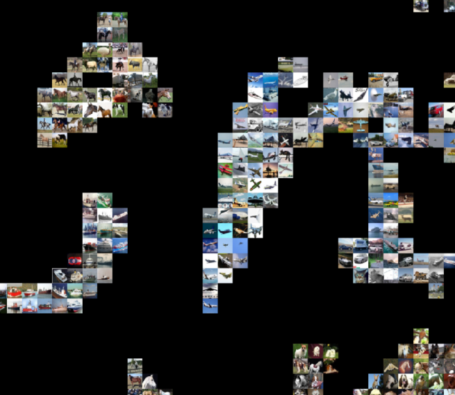
Usually we reduce the dimension to 2 for the sake of visualization in 2D space. And a common way to visualize the clustering of high-dim vectors is to create a 2D grid and use the calculated (x,y) as coordinate to position the original image. An example is shown below, the data is CIFAR10 and the features are CNN feature vectors:

tsne embedding on CIFAR10 CNN features

And a zoomed in version of a corner; the dataset is pretty well-clustered:

zoomed in

Based on the tsne embedding, you are able to evaluate your trained network, whether the learned features represent the  images in the correct way as you want. Also, you are able to tell the mis-classified data. But since this is a low dimension representation, the distance shown here doesn’t necessarily reflects the real distance between clusters.

A well-written code in MATLAB is kindly provided by Alex Karpathy in his tSNE JS demo page:  Tsne JS demo

Happy embedding!