[Linux] Chmod

I encountered the ‘access restriction’ problem when I tried to host a local webpage on to my department’s server.

The problem was that all my images inside the .html file had broken link. (where the annoying broken image icon:  shown everywhere across your website) I double checked my image directory in the .html file and there was nothing wrong with it.

Later I figured out it was the permission of my folder and files problem. It turned out that you CANNOT (at least I’m not sure how) modify the permissions or inspect what the permission of non-users are by right clicking the file/folder and checking ‘Get Info‘ on Mac. You need to use the terminal for that. And it’s all about the Chmod tricks.

Chmod stands for ‘change mode’. It modifies the access permissions to file system objects. The basic syntax is:

chmod [options] file

where ‘options’ is a 10-bit binary 9876543210; if denote the rightmost digit as index 0, then 0, 1, 2 bits control permission of other users, 3, 4, 5 bits control permission of the group, and 6, 7, 8 bits control permission of the user. 10th bit is optional. Each of the three bits represent ‘r’ for read, ‘w’ for write and ‘x’ for execute. An illustration is shown below:

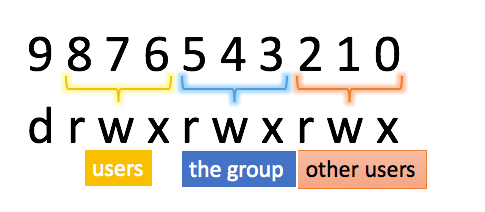
Basically, if you want to allow for ‘r’ for user, then you go to the three bits that control user permission (6, 7, 8 bits) and set 8th bit to one since it controls ‘r’.

Assume we want to change permission of a file to 1) user being able to read, write and execute, 2) group and other users being able to read only. Then we set 2, 5 to one (‘r’ for other users and the group) and 8, 7, 6 to all ones (for user to read, write and execute). Then the 10 bit binary is: 0111100100, which is equivalent as writing in 744 (111–7, 100–4, 100–4).

Instead of using numbers to denote the permission mode, we can also use ‘r’, ‘w’, ‘x’, etc. directly. ‘u’ for user, ‘g’ for group and ‘o’ for others. For example, ‘u+x’ means user is able to execute, ‘o+r’ means others can read.

chmod u+rwx filename

is the same as

chmod 700 filename

If you then want to inspect on what files have what permission, go to your file directory and type:

ls -l filename

Then you are able to figure our why certain images/files are not able to open, and what permissions you have over those files.

[Caffe] HDF5 Layer

I have struggled with HDF5 data layer when I wanted to have a vector label for each of my data. Below I will share some of my experience with this data layer that is very data-flexible but less straightforward to use.

Note that HDF5 data layer doesn’t support data transformation. This means that you have to either pre-process your data in the desired way before feeding them in, or add some additional processing layer such element-wise multiplication layer for data scaling.

Overall, HDF5 data layer requires a .h5 file and a .txt file. The .h5 file contains your data and label, while the .txt file specifies the path(s) to the .h5 file(s).

Following is an example of creating the .h5 file and its corresponding .txt file using python:

import h5py
import os
from __future__ import print_function

DIR = "/PATH TO xxx.h5/"
h5_fn = os.path.join(DIR, 'xxx.h5')

with h5py.File(h5_fn, 'w') as f:
   f['data'] = X

   f['label1'] = Y1

   f['label2'] = Y2

text_fn = os.path.join(DIR, 'xxx.txt')
with open(text_fn, 'w') as f:
   print(h5_fn, file = f)

Now you should have a .txt file and a .h5 file in your specified path.

The keys ‘data’, ‘label1’, ‘label2’ are keywords you defined for your data. You can have an arbitrary number of keywords, as long as you write the same keywords when you feed in your data to the hdf5 data layer. An example hdf5 data layer is like this:

layer {
   name: "example"
   type: "HDF5Data"
   top: "data"
   top: "label1"
   top: "label2"

   hdf5_data_param {
     source: "/PATH TO .txt file/"
     batch_size: 100
   }
}

Notice that the top blobs have the same keywords as when I created the .h5 file.

That’s it! Now you can use hdf5 data layer 🙂

[CAFFE] Resume training from saved solverstate

It’s always good to record training states so that you can always get back to the state to resume training or to use the weights from that state’s caffe model. Caffe allows you to do that by specifying some parameters in the solver prototxt file:

# The maximum number of iterations
max_iter: 6000
# snapshot intermediate results
snapshot: 2000
snapshot_prefix: "/PATH to snapshot files/"

This will save a caffemodel file and a solverstate file per snapshot. The caffemodel file contains all the trained weights of your network architecture, while the solverstate file contains the information to be used for resuming training.

If you want to resume training from a state, write a bash file like this:

#!/usr/bin/env sh
TOOLS=./build/tools
$TOOLS/caffe train \
--solver=/PATH to solver.prototxt/ \
--snapshot=/PATH to .solverstate file/

Don’t forget to change the access permission to make the bash file executable:

chmod u+x {your bash file}

[Deep Learning] T-sne Visualization

T-sne is a dimensionality reduction technique based on clustering. It’s well suited for embedding high-dimensional data, thus useful to visualize high-dim feature vectors output from deep neural networks. (Similar to PCA but more robust)

Usually we reduce the dimension to 2 for the sake of visualization in 2D space. And a common way to visualize the clustering of high-dim vectors is to create a 2D grid and use the calculated (x,y) as coordinate to position the original image. An example is shown below, the data is CIFAR10 and the features are CNN feature vectors:

tsne embedding on CIFAR10 CNN features

And a zoomed in version of a corner; the dataset is pretty well-clustered:

zoomed in

Based on the tsne embedding, you are able to evaluate your trained network, whether the learned features represent the  images in the correct way as you want. Also, you are able to tell the mis-classified data. But since this is a low dimension representation, the distance shown here doesn’t necessarily reflects the real distance between clusters.

A well-written code in MATLAB is kindly provided by Alex Karpathy in his tSNE JS demo page:  Tsne JS demo

Happy embedding!

 

[CAFFE] Data Layer

Caffe has multiple input data types, and here I will address the use of .txt file as ‘image data layer’ and lmdb as ‘data layer’. The difference between reading from .txt file that includes image paths, and reading from lmdb file format is that the former reads directly from disk while the latter allocates memory on GPU and reads from there, thus it’s pretty obvious that lmdb allows for faster training. However lmdb requires a big chuck of GPU memory allocation and is not practical when the data is huge. So there is a tradeoff.

1. txt file

Notice that .txt file corresponds to a ‘ImageData’ layer, and the keyword ‘image_data_param’. Be careful when switching between using lmdb and .txt file for inputs, you have to change these keywords correspondingly.
Here is an example of what an ‘ImageData’ layer looks like in a training prototxt file.

  name: "data"
  type: "ImageData"
  top: "data"
  top: "label"
  include {
    phase: TRAIN
  }
  transform_param {
    ...
  }
  image_data_param {
    source: "/SOURCE PATH/train.txt"
    root_folder: "/ROOT PATH/"
    shuffle: true
  }
}

and an example of what a train.txt file looks like:

train/00000001.jpg 0
train/00000002.jpg 0
train/00000003.jpg 0
...

Several important points to notice:
1) Usually the path specified in the .txt file is a relative image path to the .txt file. If that’s the case, then you have to specify the root_folder field inside ‘image_data_param’ to be the root path relative to the caffe root folder. Most of the time SOURCE PATH is the same as ROOT PATH if you put your training image folder and the train.txt file in the same folder.
2) Default parameter says shuffle to be false, so you have to explicitly make it true if you want to shuffle your data.

2. lmdb file

lmdb stands for “Lightning Memory-Mapped Database”, a key/value storage engine.

Caffe offers tool to convert to lmdb file format from multiple data formats including .bin, np arrays and .txt file. The advantage of using lmdb is the speed of training, but the downside is the memory requirements for your GPU, and if it complains about ‘out of memory’ you may have to reduce your batch size.

Different from .txt file format, lmdb format corresponds to ‘Data’ layer, and the keyword ‘data_param’. Here is an example of what a ‘Data’ layer looks like in a training prototxt file.

layer {
  name: "data"
  type: "Data"
  top: "data"
  top: "label"
  include {
    phase: TRAIN
  }
  transform_param {
    ...
  }
  data_param {
    source: "PATH TO/lmdb"
    backend: LMDB
  }
}

I’m not familiar with hdf5 data format, but it seems helpful if you are doing regression and have multiple labels as input.

[CAFFE] What files do you need to train your own network

The following list of files serves as an example to do your own training in Caffe.

• train.sh

If you are using bash, you will be running this script to train your network. This tells where to look for the solver prototxt, and whether to restart training from an existing ‘.solverstate’ file. Note that ‘–snapshot’ is optional; it’s used when you want to restart training from an existing state.

TOOLS=./build/tools        // assume you are in the caffe directory
$TOOLS/caffe train \       // the verb "train" starts the training process
--solver=<PATH TO solver prototxt>
--snapshot=<PATH TO solver .solverstate file>

• train.prototxt

This is the network architecture you define for your training.  You define all the layers you need, including data layer, convolutional layer, pooling, ReLU, etc. More examples of the prototxt file could be found in the caffe model zoo. (where trained network architecture is hosted)

The tricker component of train.prototxt is the data layer. I will have another post particularly talking about data layer later.

• deploy.prototxt

The deploy prototxt is basically a duplicate of the train prototxt. This makes sense since you want your test data to be forwarded to the same network architecture. The only difference is that you have to replace the data layer in train.prototxt with a specification of the input data dimension.

Let’s say you had this data layer in your train.prototxt

layer {
  name: "..."
  type: "Data"
  top: "data"
  top: "label"
  include {
    ...
  }
  transform_param {
    ...
  }
  data_param {
    ...
  }
}

You would want to replace the above layer with the following in your deploy.prototxt:

input: "data"
input_shape {
  dim: 1
  dim: 3 (If it's RGB color image)
  dim: Height
  dim: Width
}

• data

Caffe supports different data types to be used for training. The simplest but slowest is to use a txt file with actual image path and label written in each line. But this has a latency for data fetching from the memory, and could significantly slow down your training process.

I’m more used to using lmdb files as data source. Caffe will allocate memory onto GPU and fetch data from there, thus a big speedup for training. But it’s less straightforward creating lmdb format data file, I may have a separate post on creating lmdb format data.

After you have your data ready, you specify its path in your train.prototxt inside the data layer.

• solver.prototxt

This contains all the hyper-parameters you have for your training. An example is shown below

# The train/test net protocol buffer definition
net: "
# test_iter specifies how many forward passes the test should carry out.
# total_test_number = test_iter * batch_size
test_iter: 100
# Carry out testing every 500 training iterations.
test_interval: 500
# The base learning rate, momentum and the weight decay of the network.
base_lr: 0.001
momentum: 0.9
weight_decay: 0.004
# The learning rate policy
lr_policy: "fixed"
# Display every 100 iterations
display: 100
# The maximum number of iterations
max_iter: 4000
# snapshot intermediate results
snapshot: 4000
snapshot_format: HDF5
snapshot_prefix: "PATH TO PREFIX LOCATION"
# solver mode: CPU or GPU
solver_mode: GPU

• [optinal] solver2.prototxt

If you want to decay your learning rate after a certain amount of training iteration, you would specify another solver prototxt here with reduced learning rate. This file is optional and is only needed when you want to restart your training with a different set of hyper-parameters.

 

Basically, this is all you need to train your network with caffe. Happy brewing!

[MATLAB] Retrieve data from .fig files

In MATLAB, when you saved an image into a .fig file and then want to retrieve the data from it, you can do as follows:

First, get a handle to the input .fig image by either doing

open('display.fig');
h = gcf;  % handle to the current displayed image.

or do (relate .fig format to .mat format):

h = hgload('display.fig');   % also give you the handle to the figure file

Now h is the handle to your image file. When you close the window of the displayed image, h is deleted.

Next step is to go down the hierarchy from the figure handle –> axes object –> image object (contains the data you need)

axesObjs = get(h, 'Children');       % get the axes object from the handle
imageObj = get(axesobj, 'Children')  % get the image object from the axes object

Now that you have your image object, you are able to retrieve all source of information of your .fig image file. Within this ‘imageObj’ object, some major information:

XData: the x-dimension size of your image
YData: the y-dimension size of your image
CData: this is the matrix of your image pixel intensities

There are other properties stored in the image object such as transparency, etc. But most of the time we care about the size and content of our image file. Last step is to retrieve the info you need using the ‘get’ function:

image = get(imageObj, 'CData'); % give you the image data

The second argument could be any property contained in the image object. (e.g. XData, YData, CData, etc.)

[MATLAB] Dealing with high dimensional data in MATLAB

Ran across this problem when trying to simulate IPF–iterative proportional fitting for my STATS HW.

I was trying to construct a 7-dimensional matrix that represents clique potentials for 7 nodes. I found little resources on the web talking about dealing with high dimensional matrices in MATLAB (e.g. index specification, dimension expansion/reduction). So I just want to share some of the tricks/approaches we can use when having high dimensional (N>3) data in MATLAB.

I’m sure that there should be better solutions to address what I’m posting here, and any sharing and comment would be greatly appreciated.

Imagine we have a 2 by 2 by 2 by 2 by 2, a 5-dimensional matrix A, in MATLAB,

size(A)

would return

2 2 2 2 2

It’s usually simple to think of or visualize 2 or 3 dimensional data; but it’d be hard to create a high dimensional data image in mind.

• How to automate the process of extracting only the n^th dimension from A?

If we have a 2D matrix:

B = [1,2;3,4]

B(:,1)

would give us all the elements in the first dimension of B, in this case it’s

[1 2]

It’s not hard to think that for higher dimension that still works.

A(:,1,1,1,1)

would give us all the elements in the first dimension of A. Then the problem comes when we want to automate this extraction process. How can we make this into a for loop? There is a rather complicated way to do this. It works, but I’m sure that there could be better solutions. Hope someone can point it out.

We first create a cell with length same as the matrix dimension. This cell would store the index string we are creating.

ind = cell{1,5}

Use a for loop to set all values to

for i = 1:5
  ind{i} = {[1]};
end

The brace and brackets are important here. Each element within the cell array is a cell. Then we set the dimension we want to address to have the character:

':'
ind{dimension_addressed} = {':'};

The last step is to use this cell array to address the specific dimension we are referring to:

A(ind{:})

would be the correct way to automatically address the desired dimension in a high dimensional matrix in MATLAB.

Feature Matching in Android

The feature matching algorithm in this tutorial is in JAVA with OpenCV4Android.

My purpose of writing the code is to find the perspective transformation between a pattern and an object in a scene. Basic steps to find a homography include 1) keypoint calculation 2) descriptor calculation 3) coarse matching 4) finer matching and 5) finding the transformation matrix. ( Let’s assume that the pattern has some nice features, and that we are dealing with gray-scale images )

First of all, we have to decide what feature to use for keypoint and descriptor calculation. It’s preferred to use SIFT or SURF features but they are not compiled with OpenCV4Android as they are non-free libraries. If you don’t want to separately compile those libraries, you could alternatively use FAST or ORB features; they also work decently. And for matching algorithm, Hamming distance/L1/L2 are usually preferred options.

FeatureDetector Orbdetector = FeatureDetector.create(FeatureDetector.ORB);
DescriptorExtractor OrbExtractor = DescriptorExtractor.create(DescriptorExtractor.ORB);
DescriptorMatcher matcher = DescriptorMatcher.create(DescriptorMatcher.BRUTEFORCE_HAMMING);

For each of the two images (pattern and scene), we calculate its keypoints and descriptors

Mat descriptors1 = new Mat();
MatOfKeyPoint keypoints1 = new MatOfKeyPoint(); 
Orbdetector.detect(image1, keypoints1);
OrbExtractor.compute(image1, keypoints1, descriptors1);

Then we do matching between the two sets of descriptors of the two images. Before this step, it’s better to check the size of descriptor1 and descriptor2 to see if they have enough points

MatOfDMatch matches = new MatOfDMatch();
matcher.match(descriptors1,descriptors2,matches);

We want to discard some of the poor matches, and thus we set a threshold and only store matches that have a distance below the threshold

 LinkedList<DMatch> good_matches = new LinkedList<DMatch>();
 MatOfDMatch gm = new MatOfDMatch();
 for (int i=0;i<descriptors2.rows();i++){
   if(matchesList.get(i).distance<3*min_dist){ // 3*min_dist is my threshold here
     good_matches.addLast(matchesList.get(i));
   }
 }
 gm.fromList(good_matches);

Once we got a list of good matches, we can extract these pairs of points from the two images. If you want to match image1 to image2 (or find the transformation matrix from image1 to image2), then trainIdx is used for image1 while queryIdx is used for image2

LinkedList<Point> objList = new LinkedList<Point>();
LinkedList<Point> sceneList = new LinkedList<Point>();
for(int i=0;i<good_matches.size();i++){
  objList.addLast(keypoints2_List.get(good_matches.get(i).trainIdx).pt);
  sceneList.addLast(keypoints1_List.get(good_matches.get(i).queryIdx).pt);
}

The inputs to the function “getPerspectiveTransform” have to be in Mat format, convert the linked list to Mat formats and then find the transformation matrix between the two sets of good matching features

obj.fromList(objList);
scene.fromList(sceneList);
Mat perspectiveTransform = Imgproc.getPerspectiveTransform(obj,scene);

[Installation]Installing OpenCV 2.4.10 on Yosemite

Newest version of OpenCV 2.4.10 is out and ready for download!

Check if Xcode is installed

First check if Xcode is installed on your machine. To do that, open a Terminal and type:

$ xcode-select -p

This gives you the path to your installed xcode. If you see

$ /Applications/Xcode.app/Contents/Developer/

Your xcode is fully installed! You can also check the version of your xcode by typing:

$ /Applications/Xcode.app/Contents/Developer/usr/bin/xcodebuild -version

Download a Package Manager

Multiple package managers do the job. (e.g. Macports, Fink or Homebrew). In my case I used Macports, so everything below is based on Macports. You can check to see if it installed successfully by opening your terminal and typing:

$ port

Use Macports to get cmake

In your terminal, type in the following:

$ sudo port install cmake

This will go fetch cmake and its dependencies and install them onto your system. You can check to see if cmake is installed by typing

$ cmake

Download and Build OpenCV

Sometimes opencv.org just failed to load. I downloaded the latest OpenCV from SourceForge. (They update it so you always get the newest version!)

Download the .zip file and unzip it to a directory. We are going to build OpenCV using cmake. In terminal, go to the directory where OpenCV was extracted to. Type in the following to make a separate directory for building purpose:

mkdir build
cd build
cmake -G "Unix Makefiles" ..

Notice that there is a space before the two ending dots.

Now, we can make OpenCV. Type the following in:

make -j8
sudo make install

This should now build OpenCV into your /usr/local/ directory.

If you want to double check to ensure it is installed, go to the directory /usr/local/lib (to do this, click the ‘Go’ tab at the top of your screen and click ‘Go to folder’ to type in the directory). Clean up the files by ‘Date Modified’, you can see those **2.4.10.dylib files.

Congratulations! Now you can do a bunch of super duper cool stuff with this awesome vision tool.